cometsuite
Cometary dust dynamics simulator.
Contents:
Quick start
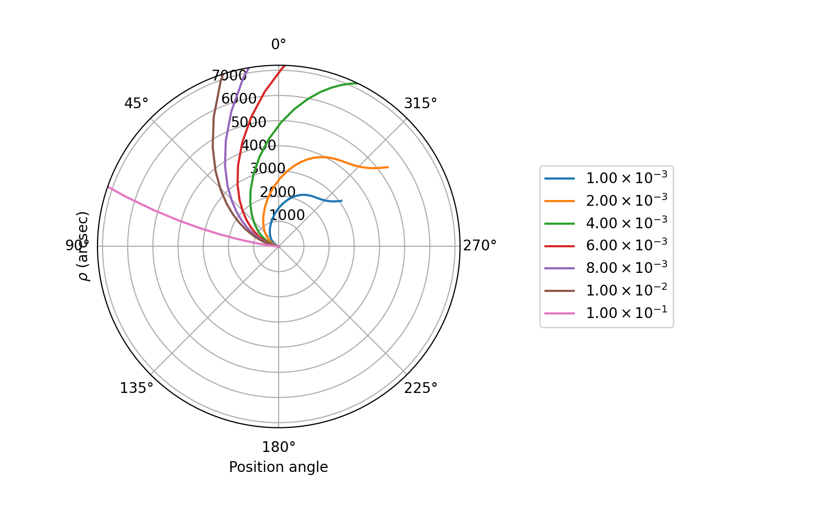
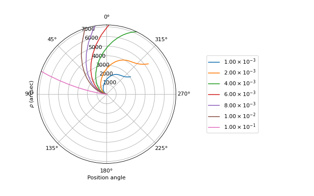
Syndynes
Reproduce the syndynes of Reach et al. (2000) for comet 2P/Encke:
>>> import numpy as np
>>> import matplotlib.pyplot as plt
>>> from astropy.time import Time
>>> from mskpy import KeplerState
>>> import cometsuite as cs
>>>
>>> # observation date, comet's position and velocity in km and km/s
>>> date = Time(2450643.5417, format="jd")
>>> rc = [4.36955224e7, -1.64073549e8, -2.73990869e7]
>>> vc = [26.40398803, -21.02309023, -1.63325062]
>>>
>>> # and the vectors for the observer (Earth)
>>> re = [5.61856527e7, -1.41307139e8, -1.23261993e3]
>>> ve = [2.71884498e1, 1.09043893e1, -6.22859821e-04]
>>>
>>> # KeplerState generates vectors based on Keplerian (two-body) propagation
>>> comet = KeplerState(rc, vc, date, name="Encke")
>>> earth = KeplerState(re, ve, date, name="Earth")
>>>
>>> # generate syndynes for each of these β values, a 200 day length, and 101 time steps
>>> beta = [0.001, 0.002, 0.004, 0.006, 0.008, 0.01, 0.1]
>>> ndays = 200
>>> steps = 101
>>>
>>> # quick_syndynes is, by default, Kelperian-based
>>> sim = cs.quick_syndynes(comet,
...                         date,
...                         beta=beta,
...                         ndays=ndays,
...                         steps=steps,
...                         observer=earth)
>>> ax = plt.gca()
>>> plt.setp(ax,
...          xlabel='Position angle',
...          ylabel=r'$\rho$ (arcsec)',
...          rmax=(2 * 3600))  # 4 degree FOV
(Source code, png, hires.png, pdf)
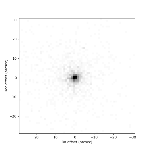
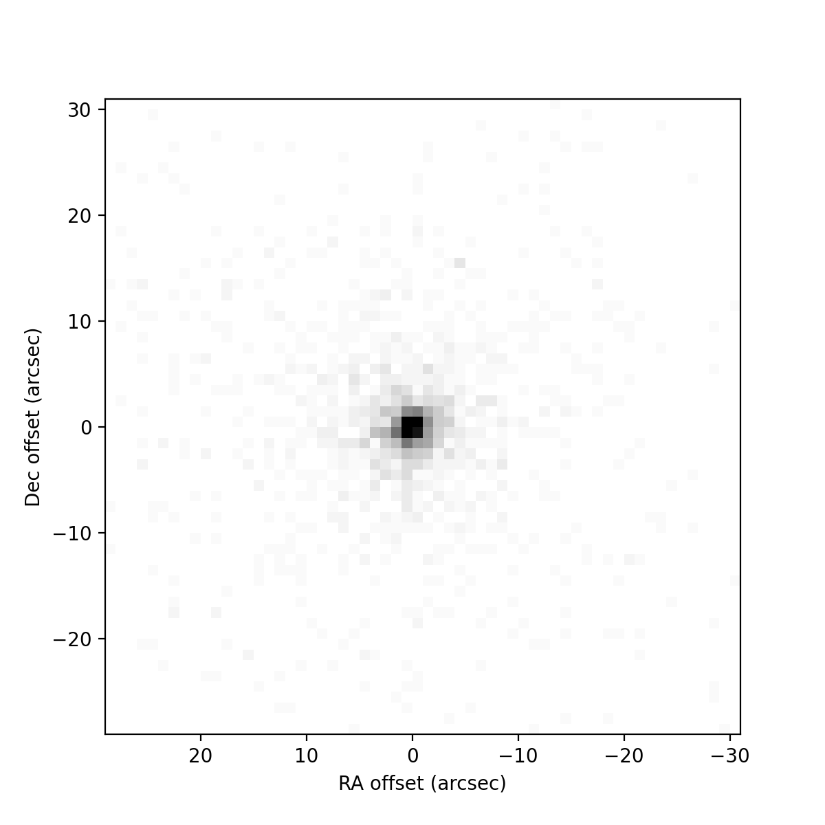
Monte Carlo Coma
Simulate the coma for T-ReCS observations of C/2009 P1:
>>> import matplotlib.pyplot as plt
>>> from astropy.time import Time
>>> from mskpy import KeplerState
>>> import cometsuite as cs
>>> import cometsuite.generators as gen
>>> import cometsuite.scalers as sc
>>>
>>> # observation date, position (km) and velocity (km/s) of
>>> # comet and observer
>>> date = Time("2011-09-11")
>>> # comet:
>>> rc = [1.99512556e8, -1.86957354e8, 1.49657485e8]
>>> vc = [-23.28613574, 10.86086487, 13.85289671]
>>> # Earth:
>>> re = [1.47206597e8, -3.19139879e7, 1.38953505e2]
>>> ve = [5.82028904e+00,  2.89897439e+01, -1.16199526e-03]
>>>
>>> # two-body orbit propagation
>>> comet = KeplerState(rc, vc, date, name="C/2009 P1")
>>> earth = KeplerState(re, ve, date, name="Earth")
>>>
>>> # particle generator and parameters
>>> #   - geometric "composition": beta = 0.57 / a / rho
>>> #   - particle ages up to 5 days
>>> #   - sizes from 0.1 μm to 1 mm
>>> #   - isotropic dust production from a point source nucleus
>>> #   - speed = 0.3 rh**-0.5 a**-0.5 (km / s)
>>> # generate 2,000 particles
>>>
>>> pgen = cs.Coma(comet, date)
>>> pgen.composition = cs.Geometric(rho0=1)
>>> pgen.age = gen.Uniform(0, 5)
>>> pgen.radius = gen.Log(-1, 3)
>>> pgen.vhat = gen.Isotropic()
>>> pgen.speed = gen.Delta(0.3)
>>> pgen.speed_scale = sc.SpeedRh(-0.5) * sc.SpeedRadius(-0.5)
>>> pgen.nparticles = 2000
>>>
>>> # generate and integrate particle positions
>>> integrator = cs.BulirschStoer()
>>> sim = cs.run(pgen, integrator)
>>>
>>> # project particle positions onto the sky
>>> sim.observer = earth
>>> sim.observe()
>>>
>>> # image with a 60x60 pixel camera, 1"/pixel
>>> camera = cs.Camera(size=(60, 60), cdelt=[-1, 1])
>>> camera.integrate(sim)
>>>
>>> fig, ax = plt.subplots(figsize=(6, 6), dpi=200)
>>> ax.imshow(camera.data, vmin=0, vmax=50, cmap="gray_r", extent=[30, -30, -30, 30], origin="lower")
>>> plt.setp(ax, xlabel="RA offset (arcsec)", ylabel="Dec offset (arcsec)")
>>> plt.tight_layout()
(Source code, png, hires.png, pdf)
